EFFECT OF DISTURBANCE ON SOIL

COMPOSITION AND CHARACTERISTICS OF SOIL

The scientific study of soil is called pedology. Soil is composed of both organic and inorganic matter, and it is essential for life on earth to exist. The soil type that i have studied is brown earths. Brown earths are the most common soil type in Ireland and are very fertile. Soils are a composition of mineral particles 45% , organic matter 5% , air 25% , and water 25% .

Mineral Particles:
Mineral particles are the largest ingredient and make up approx 45% of soils . They are the original rock that got broken down by weathering and erosion to form the basis of soil. The type of rock that was broken down to form it is called the parent rock. The broken down rock produces minerals such as calcium, phosphorus, and potassium in the soil on which the plants feed. The parent material influences the soil colour, depth, texture and ph value 

Organic Matter:
Organic matter is decayed vegetation that is broken down by micro organisms in the soil to form humus . Humus is a dark jelly like substance that binds the soil together and improves its texture. It increases the soils ability to retain moisture. Brown earths develop in area of deciduous woodland where there is an abundance of plant litter available to decay. Brown earth soils are also found where temperatures average zero for less than 3 months of the year and rarely exceed 21 degrees. These conditions allow for microorganisms to thrive. The colour of the soil is an indication of the amount of organic material it contains with darker soils having more organic content. Humus is plentiful in brown earths

Air and Water: 
Air is vital for the survival of micro-organisms and without theses, there would be a shortage of humus. Brown earths have a granular structure which allow for good aeration. Plants cannot survive without water present in the soil .Mineral particles are soluble in water and the roots of plants can only absorb the nutrients of them after they have been dissolved 
Characteristics of brown earths :
Brown earths are usually 2 metres deep and have 4 horizons . The A horizon has a thick layer of dark humus. There is a plentiful supply of micro organisms which mix the soil well and leave no distinct boundary between the A and B horizons. The B horizon is similar but with a lighter brown colour. The C horizon has a n accumulation of clay and broken down rock. The bottom layer is the bedrock 
Brown earths are fertile and very suitable for agriculture. Their suitability for agriculture are due to their characteristics of good texture, dark colour, and ph value .


Texture: 
Texture is how a sol feels when you touch it. The proportions of sand silt and clay determines the soils texture. The texture determines how well moisture and roots can penetrate the soil and how well excess moisture can drain away. The ideal combination for soil texture is roughly 40% sand, 40% silt, and 20% clay creating what is known as a loam soil. Brown earths fall into this category. They have a well-developed crumb structure which allows water air and organisms pass through it easily, and roots can spread out in it easily. Water retention is good as it is soaked up by the crumbs of the soil and nutrient retention is good also. They also have good drainage and aeration properties. Loam soils such as brown earths are ideal for cultivation

Colour: 
Lighter coloured soils deflect sunlight while dark soils absorb more light. This allows the soil to heat up much more quickly and encourages seed germination and crop growth, Heat is also important in the humification process. Brown earths have a high humus content which makes it a darker soil and thus supports good crop growth 

PH Value: 
PH scale measure the acidity of a substance. The ideal PH value for agriculture is 6.5 which is slightly acidic. A soil which is too acidic lacks calcium and potassium which are essential for growth and has low levels of organisms which are vital for humification. Soils which are quite acidic are peaty soils which have a ph value of less than 4and are found mainly in the mountainous areas of the west. They have suffered from leaching and tend to be waterlogged also. Brown earths have a ph value of between 5 and 7, ideal values that are known to be very fertile supporting a wide variety of plant life

CHARACTERISTICS OF CLAYS

Clays and clay minerals have been mined since the Stone Age; today they are among the most important minerals used by manufacturing and environmental industries. The U.S. Geological Survey (USGS) supports studies of the properties of clays, the mechanisms of clay formation, and the behavior of clays during weathering. These studies can tell us how and where these minerals form and provide industry and land-planning agencies with the information necessary to decide how and where clay and clay mineral deposits (fig. 1) can be developed safely with minimal effects on the environment.

The term “clay” is applied both to materials having a particle size of less than 2 micrometers (25,400 micrometers = 1 inch) and to the family of minerals that has similar chemical compositions and common crystal structural characteristics (Velde, 1995) described in the next section. Clay minerals have a wide range of particle sizes from 10’s of angstroms to millimeters. (An angstrom () is a unit of measure at the scale of atoms.) Thus, clays may be composed of mixtures of finer grained clay minerals and clay-sized crystals of other minerals such as quartz, carbonate, and metal oxides. Clays and clay minerals are found mainly on or near the surface of the Earth.

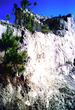
Figure 1. Massive kaolinite deposits at the Hilltop pit, Lancaster County, South Carolina; the clays formed by the hydrothermal alteration and weathering of crystal tuff. Pine tree in the foreground is about 2 meters in height.

Physical and Chemical Properties of Clays

The characterististics common to all clay minerals derive from their chemical composition, layered structure, and size. Clay minerals all have a great affinity for water. Some swell easily and may double in thickness when wet. Most have the ability to soak up ions (electrically charged atoms and molecules) from a solution and release the ions later when conditions change.

Water molecules are strongly attracted to clay mineral surfaces. When a little clay is added to water, a slurry forms because the clay distributes itself evenly throughout the water. This property of clay is used by the paint industry to disperse pigment (color) evenly throughout a paint. Without clay to act as a carrier, it would be difficult to evenly mix the paint base and color pigment. A mixture of a lot of clay and a little water results in a mud that can be shaped and dried to form a relatively rigid solid. This property is exploited by potters and the ceramics industry to produce plates, cups, bowls, pipes, and so on. Environmental industries use both these properties to produce homogeneous liners for containment of waste.

The process by which some clay minerals swell when they take up water is reversible. Swelling clay expands or contracts in response to changes in environmental factors (wet and dry conditions, temperature). Hydration and dehydration can vary the thickness of a single clay particle by almost 100 percent (for example, a 10-thick clay mineral can expand to 19.5 in water (Velde, 1995). Houses, offices, schools, and factories built on soils containing swelling clays may be subject to structural damage caused by seasonal swelling of the clay portion of the soil.

Another important property of clay minerals, the ability to exchange ions, relates to the charged surface of clay minerals. Ions can be attracted to the surface of a clay particle or taken up within the structure of these minerals. The property of clay minerals that causes ions in solution to be fixed on clay surfaces or within internal sites applies to all types of ions, including organic molecules like pesticides. Clays can be an important vehicle for transporting and widely dispersing contaminants from one area to another.

How and Where Clays and Clay Deposits Form

Clays and clay minerals occur under a fairly limited range of geologic conditions. The environments of formation include soil horizons, continental and marine sediments, geothermal fields, volcanic deposits, and weathering rock formations. Most clay minerals form where rocks are in contact with water, air, or steam. Examples of these situations include weathering boulders on a hillside, sediments on sea or lake bottoms, deeply buried sediments containing pore water, and rocks in contact with water heated by magma (molten rock). All of these environments may cause the formation of clay minerals from preexisting minerals. Extensive alteration of rocks to clay minerals can produce relatively pure clay deposits that are of economic interest (for example, bentonites却rimarily montmorillonite丘sed for drilling muds and clays used in ceramics).

Erosion

The transport and deposition of clays and clay minerals produced by eroding older continental and marine rocks and soils are important parts of the cycle that forms sedimentary rocks. The ancient sedimentary rock record is composed of about 70 percent mudstones (which contain about 50 percent clay-sized fragments) and shales (which are coarser than mudstones but which may contain clay-sized particles) (Blatt and others, 1980). Today, sedimentary environments that contain muds cover about 60 percent of marine continental shelves and 40 percent of deep ocean basins; continental aquatic environments such as lakes, rivers, estuaries, and deltas also contain high proportions of fine-grained sediments (Hillier, 1995, p. 162). Clearly, clays and clay minerals are critical components of both ancient and modern sedimentary environments.

Diagenesis

Diagenesis is the in-place alteration of a mineral to more stable forms, excluding surficial alteration (which is weathering); diagenesis occurs, for example, when minerals stable in one depositional environment are exposed to another by burial and compaction. Common silicate materials such as quartz, feldspars, and volcanic glasses, as well as carbonates, noncrystalline iron oxides, and primary clay minerals, are transformed during diagenesis into more stable clay minerals mainly by dissolution and recrystallization.

The formation of bentonite (beds containing smectite-group clay minerals including montmorillonite) and fuller’s earth (a type of clay mineral deposit that has high capacity to absorb water) may occur primarily by diagenesis, although some deposits may also form by hydrothermal processes. Bentonite beds usually form from altered volcanic ash, but other types of rock may also serve as sources. The absorptive properties of bentonites and fuller’s earth make them ideal for such diverse uses as drilling mud; foundry-sand bond; binder for pelletizing iron ore and bleaching liquids; absorbents for oil, grease, and animal waste; and carriers for pesticides and fertilizers. Bentonite is also used as a soil liner for environmental containment applications and with polyacrylamide for making paper.

Weathering

Weathering of rocks and soil is the primary way that clays and clay minerals form at the Earth’s surface today. The weathering process involves physical disaggregation and chemical decomposition that change original minerals to clay minerals; weathering is uneven, and many stages of breakdown may be found in the same clay sample. Factors governing rock weathering and soil formation include the initial type of rock, the ratio of water to rock, the temperature, the presence of organisms and organic material, and the amount of time. The types of clay minerals found in weathering rocks strongly control how the weathered rock behaves under various climatic conditions (such as humid-tropical, dry-tropical, and temperate conditions).

Kaolinite is found in most weathering zones and soil profiles. Montmorillonites, which are chemically more complex than kaolinites, are common in the lower parts of weathering profiles, nearer the rock, where chemistry exerts a strong control on mineralogy. Complex mixed-layer clay minerals (such as illite-smectites) are abundant in clay assemblages that develop from mica-bearing precursor rocks, such as the granite plutons that occur in temperate regions of the Northeastern United States. For example, a large component of soils formed by weathering of granites may consist of metastable muscovite, biotite, and chlorite. These minerals will alter progressively to clay minerals.

Environmental Studies

Industrial minerals, such as clays, sand, gravel, and crushed stone, are raw materials used for building and maintaining infrastructure, agriculture, and mitigation of environmental problems. Because of the many uses for industrial minerals in our society, land management agencies have an increasing need for better geologic and mineralogic data on industrial minerals. The USGS supports studies to understand the geology of these deposits, the surficial environments, and the processes by which these deposits form.

The USGS and industry cooperators are initiating petrologic, mineralogic, and geochemical studies to better determine how economic clay deposits form. A special emphasis of these studies is to characterize the weathering portion of the life cycle of a clay deposit.

Regional data bases (such as the Southeastern United States clay deposit data base) are being developed that contain geologic and geochemical information necessary to establish environmental characteristics that affect the use of clays and clay minerals. Environmental characteristics include the nature and distribution of inorganic contaminants, such as metals and metalloids like arsenic, iron, and lead, in clay-bearing rocks. These environmental factors have the potential to affect the use of clays in natural and industrial applications.

MOHR- COLUMBS FAILURE THEORY

Mohr-Coulomb failure theory

Soil generally fails in shear. At the failure surface, shear stress reaches the shear strength (t_f) of the soil. It the failure surface, sliding between the particles takes place as shown in Figure 10.1. The resistance that the soil offers during deformation is mainly due to the shear resistance between the particles at their contact points at the failure surface. No crushing of individual particle takes place. According to Mohr-Coulomb failure criterion, the shear strength of the soil can be expressed as:

\[{\tau _f}=c + \sigma \tan \emptyset\]               (10.1)

where c is the cohesion and Ø is the angle of internal friction of the soil. σ is the applied normal stress. The line satisfying the Eq. (10.1) is called the Mohr-Coulomb failure envelop (as shown in Figure 10.2 with red color). In Figure 10.2, it is shown that t_f is the maximum stress soil can take without failure under an applied vertical stress σ  (with blue color). Figure 10.3 shows the Mohr circle of two soil elements one at the failure surface (red color) and one at any other location (blue color). The Mohr circle touches the failure envelop incase of soil element taken from location of failure surface, whereas Mohr circle of the soil element taken from other than the location of failure surface is situated below the failure envelop. Keeping σ₃constant, if vertical stress (σ₁) increases the Mohr Circle becomes larger and finally it will touch the failure envelop and failure will take place (as shown in Figure 10.4). Figure 10.5 shows the Mohr circle for total stress and effective stress condition. The Eq. (10.1) represents the shear strength in terms of total stress (σ). In terms of effective stress (σ’ = σ – u), the shear strength of the soil can be expressed as:

where u is the pore water pressure.

Fig. 10.1. Failure surface and shear resistance.

Fig. 10.2. Mohr-Coulomb failure criterion and failure envelop.

Fig.10.3. Mohr circles of different soil elements

Fig. 10.4. Mohr circles for different stress condition

Fig. 10.5. Mohr circles for total stress and effective stress conditi

STRENGTH PARAMETERS OF SOIL

Determination of Strength parameters  

The shear strength parameters cohesion (c) and friction angle (Φ) can be determined by different laboratory tests for different types of soils.

Direct shear test:   

The soil sample is tested in a confined metal box of square cross-section. The box has two halves horizontally and a small clearance is maintained between them. Figure 10.1 shows a direct shear test set-up. Upper half of the box is fixed and lower half of the box is pushed or pulled horizontally with respect to the fixed half. Thus, a shear is applied in the soil sample. A constant normal force (vertical) is applied on the sample throughout the test. Then horizontal force or shearing is applied till the failure. The shearing is normally applied at a constant rate of strain. The amount of shear load is measured with the help of proving ring. The vertical as well as horizontal deformation is measured with the help of dial gauges. The test procedure is repeated for different normal stresses (four to five normal stresses). The shear stress at failure is plotted against different normal stresses (as shown in Figure 11.2). The shear strength parameters are determined from the best-fit straight line passing through the test points (as shown in Figure 11.2). The test is suitable for sandy soils. If the sample is partially or fully saturated, porous stones are placed below and top of the sample to allow free drainage. Figure 11.3 shows typical shear stress-shear displacement and change in height of sample-shear displacement plot of soils obtained from direct shear tests.

Fig. 11.1. Direct shear test

Fig. 11.2. Shear stress-normal stress plot

Fig. 11.3. Shear stress-shear displacement and change in height of sample-shear displacement plot of soils obtained from direct shear tests.

Unconfined compression test

The test is suitable for saturated clay (Ø_u =0). The test is conducted under zero cell pressure. Thus, it a special case of triaxial test with σ₃ = 0 (triaxial test is described in lesson 12). A cylindrical specimen is subjected to axial stress until failure. Figure 11.4 shows the Mohr circle for unconfined compression test. For purely clayey soil, _Øu =0, the subscript u is used as the test is undrained test. The major principle stress (σ₁) is equal to the unconfined compressive strength of the soil (q_u).

Fig. 11.4. Mohr-Coulomb plot for an unconfined compression test on saturated clay.

 

The undrained cohesion can be determined as:

          …………………………………………………………………………………(11.1)

For determining the unconfined compressive strength of the soil (q_u) (the applied load at failure divided by the cross-sectional area of the sample), the cross-section of the soil sample at failure load (A_f) is determined as:

 ……………………………………………………………………………….(11.2)

where A₀  is the initial cross-sectional area of the sample and e is the axial strain in the sample. The strain in the sample can be determined as:

\[\varepsilon=\frac{{Change\;in\;length\;(\Delta L)}}{{Initial\;length\;of\;the\;sample\;(L)}}\]………………………………….(11.3)

The usual sizes of the samples are: 76 mm (length) x 38 mm (diameter) or 100 mm (length) x 50 mm (diameter).

References

Ranjan, G. and Rao, A.S.R. (2000). Basic and Applied Soil Mechanics. New Age International Publisher, New Delhi, India

PPT of Professor N. Sivakugan, JCU, Australia

 Suggested Readings

Ranjan, G. and Rao, A.S.R. (2000) Basic and Applied Soil Mechanics. New Age International Publisher, New Delhi, India.

Arora, K.R. (2003) Soil Mechanics and Foundation Engineering. Standard Publishers Distributors, New Delhi, India.

Murthy V.N.S (1996) A Text Book of Soil Mechanics and Foundation Engineering, UBS Publishers’ Distributors Ltd. New Delhi, India. 

STRESS PATH

13.1. What is Stress path?

Stress path is used to represent the successive states of stress in a test specimen of soil during loading or unloading. Series of Mohr circles can be drawn to represent the successive states of stress, but it is difficult to represent number of circles in one diagram. Figure 13.1 shows number of Mohr circles by keeping σ₃ and increasing σ₁ on σ  – t  plane. The successive states of stress can be represented by a series of stress points and a locus of these points (in the form of straight or curve) is obtained. The locus is called stress path. The stress points on σ  – t  plane can be transferred to p–q plane (as shown in Figure 13.1). The coordinates of the stress points on p–qplane can be obtained as:

\[p={{{\sigma _v} + {\sigma _h}} \over 2}\]                    (13.1)

\[q={{{\sigma _v} – {\sigma _h}} \over 2}\]                     (13.2)

The stress path can be drawn as:

(a) Total stress path (TSP)

(b) Effective stress path (ESP)

(c) Stress path of total stress minus static pore water pressure (TSSP)

If in a field situation, static ground water table exists, initial pore water pressure u₀ will act on the sample. Thus, the static pore water pressure will be equal to u₀. The effective stress coordinates of the stress points on p’-q’ plane can be obtained as:

\[p’={{{\sigma _v} – u + {\sigma _h} – u} \over 2} = {{{{\sigma ‘}_v} + {{\sigma ‘}_h}} \over 2}\]                     (13.3)

\[q’={{{\sigma _v} – u – ({\sigma _h} – u)} \over 2} = {{{{\sigma ‘}_v} – {{\sigma ‘}_h}} \over 2} = {{{\sigma _v} – {\sigma _h}} \over 2}=q\]             (13.4)

Figure 13.2 shows different stress paths for normally consolidated clay obtained from CU (effective) test.  

Fig. 13.1. Stress point on Mohr circle and on p-q plane.

Fig.13.2. Different stress paths.

For initial condition, σ_v =σ_h =0 and if σ_vand σ_h are increased in such as way that ratio σ_h /σ_v is constant. This ratio is called lateral stress ratio, K. Thus,

\[K={{{\sigma _h}} \over {{\sigma _v}}}\]                                                                                            (13.5)

Similarly, coefficient of lateral earth pressure at rest (K₀) and at failure (K_f) can be expressed as:

\[{K_0}={{{{\sigma ‘}_h}} \over {{{\sigma ‘}_v}}}\]                                                                             (13.6)

 
 \[{K_f}={{{{\sigma ‘}_{hf}}} \over {{{\sigma ‘}_{vf}}}}\]                                                                   (13.7)

 
On p–q plane, the stress ratios are representing straight lines (as shown in Fig. 13.3).

Fig. 13.3.  Variation of Stress Rations.

Figure 13.4 shows the relationship between K_f line (on p–q plane) and Mohr-Colomb failure envelope (on s  – t plane). The shear strength parameters can also be determined from K_f line on p–q plane as:

\[\phi={\sin ^{ – 1}}(\tan \psi )\]                      (13.8)

\[c={a \over {\cos \phi }}\]                               (13.9)

Fig. 13.4. Relationship between K_f line and Mohr-Colomb failure envelope.

 

References

Ranjan, G. and Rao, A.S.R. (2000). Basic and Applied Soil Mechanics. New Age International Publisher, New Delhi, India

PPT of Professor N. Sivakugan, JCU, Australia.

 

Suggested Readings

Ranjan, G. and Rao, A.S.R. (2000) Basic and Applied Soil Mechanics. New Age International Publisher, New Delhi, India.

Arora, K.R. (2003) Soil Mechanics and Foundation Engineering. Standard Publishers Distributors, New Delhi, India.

Murthy V.N.S (1996) A Text Book of Soil Mechanics and Foundation Engineering, UBS Publishers’ Distributors Ltd. New Delhi, India.

TIME RATE OF SETTLEMENT

When a soil is subjected to an increase in effective stress, the porewater is squeezed out in a manner similar to water being squeezed from a sponge, and the basic concepts presented above govern the time rate of settlement of the surface of a clay layer. The following sections describe the theory of onedimensional consolidation for the case of instantaneous loading. In cases where the loading of the surface of the consolidating layer of soil varies over time, more advanced analytical techniques have been developed. These advanced theories of consolidation also may include more nonlinear soil properties than the simple theory that follows.

The theory to be presented herein is Terzaghi’s theory of one-dimensional consolidation, first presented in 1923. It remains the most commonly used theory for computing the time rate of settlement, even though it contains simplifying assumptions that are not satisfied in reality. The theory yields results of satisfactory accuracy when applied to predicting time rates of settlement of embankments on soft, saturated, homogeneous clays.
Primary Consolidation Water is forced out of a porous body like a sponge by the water pressure developed inside the sponge. However, in the case of thick layers of soil, the water pressure increases with depth, as in a quiet body of water, even though no flow is present in the water. Instead, water is forced to flow by applying an external pressure to the soil, but it is not the total water pressure that governs. In a soil where no water flow is occurring, the porewater pressure is termed the static porewater pressure us and is equal to the product of the unit weight of water and the depth below the water table:

As discussed previously, the application of the load from an embankment increases the total porewater pressure and flow begins. The flow of water is caused by the part of the total pore pressure that is in excess of the static value. For convenience, the excess porewater pressure u is defined as

where u is the total porewater pressure and Us is the static water pressure. The rate of outflow of water is also controlled by how far the water must flow to exit and by the size of the openings in the soil. The average velocity of water flow in the soil v varies directly with u and inversely with flow distance L:

The total rate of water flow (flow volume per unit of time), q,is

where v is the average flow velocity and A is the cross-sectional area. Actual experiments with soils show that the flow rate varies with the permeability of the soil and that the total rate of water flow is

where k is a constant of proportionality termed the coefficient of permeability or the coefficient of hydraulic conductivity, and s is now used to indicate distance in the direction of flow. Equation 3.47 is one form of Darcy’s law, which states that water flows in response to an energy gradient in the soil.
Those familiar with fluid mechanics may also know this, as flow will occur in response to a differential in hydraulic head.
Darcy’s law is applied to the one-dimensional consolidation problem first in a qualitative sense. A clay layer is underlain by a freely draining sand (Figure 3.10). The water table is at the surface. An embankment is put into place in a very short period of time, and the total pore pressure increases by an amount yH, where 
 is the unit weight of the embankment material and H is the thickness of the embankment. Excess pore pressures are developed in the sand layers too, but the sand consolidates so fast that the excess pore- water pressure in the sand is dissipated by the time the construction of the embankment is complete, even though very little consolidation has occurred in the clay at this stage. Thus, the sand is freely draining compared with the clay, and u is set equal to zero in the sand. The initial excess porewater pressure in the clay, u0 equals yH and is independent of depth. Because only u , 0 the excess porewater pressure causes water flow, the value of u is plotted

Figure 3.10 Pore pressures in a clay layer loaded instantaneously.

versus depth, as in Figure 3.10, and the total porewater pressure, u, and the static porewater pressure, us are ignored. At the upper and lower boundaries of the clay layer (Figure 3.10) wheredrainage occurs, the original excess porewater pressure transitions between in the clay layer and zero at the boundary with the sand over a very small u 0 distance. Thus, at time zero, just after the embankment has been put in place,
the excess porewater pressure gradient, du /dz, at both drainage boundaries approaches infinity, and thus the rate of outflow of porewater is also nearly infinite (Eq. 3.47). The total outflow volume of water Q is

where t is time. Clearly, an infinite value of q can exist only instantaneously; then the flow rate drops and finally becomes zero when equilibrium is again established. The flow rate of water from the soil q decreases because the excess porewater pressure dissipates, thereby decreasing the gradient, du /dz, and the resulting flow (Eq. 3.47). The shapes of the curves of q and Q versus time must be as shown in Figure 3.11. The settlement of the surface is found by dividing Q by A, the horizontal area of the soil deposit from which the flow Q emanates. The excess porewater pressures must vary as indicated in Figure 3.12, where time increases in the order t0, t1, t2,…, t .
Development of a mathematical theory to yield numerical values for these curves requires mathematics for solution of differential equations using Fourier series. Solutions may be developed for a variety of different initial excess porewater pressure distributions. The following solution is for the case of a uniform distribution of excess porewater pressure versus depth with drainage from the upper and lower boundaries.
The settlement at any time S is equal to the average degree of consolidation U times the ultimate settlement Su:

In this equation, Su is the settlement calculated previously and U has a value between zero and unity. U is given by

where M is

e is the base of Napierian (natural) logarithms, and T is a dimensionless time factor given by

where

Cv= coefficient of consolidation,
t = time (equal to zero at the instant the embankment is put in place),
H = total thickness of the clay layer, and
n = number of drainage boundaries.

The coefficient of consolidation has units of length2/ time and is given by the equation

The following is a sample calculation of the settlement–time curve. The soil profile in this problem is a homogeneous layer of saturated clay with a thickness of 10 ft. The compressible stratum is overlain and underlain by freely draining sand layers, and the water table is at the upper surface of the clay and is assumed to remain at the interface of the compressible layer and the upper sand layer. The upper sand layer has a submerged unit weight of 70 pcf. The clay is normally consolidated and has an average water content of 40%, a compression index of 0.35, and a coefficient of consolidation of 0.05 ft 2 /day. A 15-ft-thick wide embankment is rapidly put in place. Its unit weight is 125 pcf. In this problem, the clay layer will not be subdivided into sublayers.
The solution begins with the computation of the initial void ratio, effective unit weight, and initial effective stress at the middle of the clay layer:

In lieu of using the values of T versus U in Table 3.3, values for T can be approximated for selected values of U by the following equations:

Other points on the S-t curve corresponding to different values of U are calculated in a similar way.
Calculations like those shown above are often made in engineering practice, but many settlement problems are more complex than the case with instantaneous loading that was considered. Some of the more common factors that require the application of computer-based solutions for problems of time rate of settlement occur when fill is placed and/or removed versus time, consolidation properties exhibit significant nonlinear properties, artesian conditions are affected by construction activities, and consolidation in the field
is accelerated using wick drains. Secondary Compression After sufficient time has elapsed, the curve of settlement versus logarithm of time flattens. Theoretically, the curve should become asymptotically flat, but observations both in laboratory tests and in the field find a curve with a definite downward slope. This range of settlement with time is called secondary compression and includes all settlements beyond
primary consolidation. The slope of the secondary compression line is expressed as the coefficient
of secondary compression C :

The coefficient of secondary compression is used in settlement computations  in a manner similar to that of the compression, reloading, and rebound indices, except that time is used in place of effective stress when computing the settlement:

The terms consolidation and compression are used carefully in this book. Compression includes any type of settlement due to a decrease in the volume of soil. Consolidation refers to settlement due to the squeezing of water from the soil and the associated dissipation of excess pore water pressures.

DEEP FOUNDATION

1 Introduction: Typical types of deep foundations are discussed in the following paragraphs. Entrepreneurs have developed several special and innovative types of deep foundations, and more will continue to be offered by the construction industry…

2 Driven Piles with Impact Hammer: The engineer frequently makes an extensive and thorough investigation prior to selecting of the type and configuration of a pile for a particular project…

3 Drilled Shafts: The design and construction of drilled shafts are discussed in detail in many publications (e.g., Reese and O’Neill, 1988)…

4 Augercast Piles: Augercast piles (also known as augered-cast-in-place piles) are constructed by turning a continuous-flight auger with a hollow stem into the soil…

5 GeoJet Piles: The GeoJet pile is described as an example of a special kind of deep foundation…

6 Micropiles: Micropiles are deep foundations with a small diameter. They may be installed in a variety of ways and have several purposes…

VANE SHEAR DEVICE

Field vane testing consists of inserting vanes at the ends of rods into soft, saturated soils at the bottom of a borehole and rotating the rods to find the torsion that causes the surface enclosing the vane to be sheared.

The torsion is converted into a unit shearing resistance. Two views of typical vanes are shown in Figure 4.11. If the rod used to insert the vane is in contact with the soil, a correction must be made for the torsion on the rod.

With the vane in position, the first test is performed by rotating the rod attached to the vane at a rate not exceeding 0.1º per second, usually requiring 2 to 5 minutes to achieve the maximum torque, yielding the undisturbed shear strength. Then the vane is rotated rapidly through a minimum of 10 revolutions to remold the soil. Finally, the test is repeated to obtain the remolded shear strength of the soil.

The shear strength, s (lbf / ft2), is found from the following equation:

A problem with no easy solution is one in which the soil has inclusions such as shells. The value of s from the vane would be higher than the actual shear strength and could lead to an unsafe design.

THREE PHASE DIAGRAM OF SOIL

​

Three Phase Diagram:

A soil mass consist of the solid particles and the voids in between them. These voids are filled with air or/and water.  So there is a three phase system, but when the voids are only filled with air, or only filled with water then soil becomes a two phase system.  Three phase system can be represented with a diagram as shown below. When the voids are only filled with water, it is said to be saturated.

  

Total volume of the soil mass, V = (Va+Vw) +Vs

Where, V = Total Volume

 Va= Volume of air mass

 Vw = Volume of water mass

Vs = Volume of solids

But, Va+Vw = Vv

So,

      V = Vv+ Vs

Where Vv= Total volume of voids.

Void Ratio(e):

Void ratio is the ratio of the volume of the voids to the volume of the solid in the soil.

It is denoted by ‘e’. 

e= Vv/Vs = n/(1-n)

Porosity (n): 

Porosity is defined as the ratio of the volume of the total voids to the total volume of the soil mass. 

It is denoted by ‘n’

So n = Vv/V = e/(1+e)

Degree of Saturation(Sr):

Degree of saturation is defined as the ratio of the volume of the water to the total volume of the voids present in the soil mass. 

Sr = Vw/Vv,  For fully saturated soil mass Vw=Vv, So Sr=1

                      For fully dry soil mass, Vw= 0, So Sr=0

Water content(w):

It is the ratio of the weight of the water to the weight of the solids in the given soil mass. Weight of solids can be found by weighing the soil mass after drying it completely.

   w = Ww/Ws

Air Content(na): 

It is the ratio of the volume of air(Va) to the total volume of the voids(V).

   na= Va/V*100